Nesterov Momentum meets Neural Ordinary Differential Equations
Published:
Our work at NeurIPS 2022, titled “Improving Neural Ordinary Differential Equations with Nesterov’s Accelerated Gradient Method,” focuses on improving the efficiency of Neural Ordinary Differential Equations, which is a recent type of machine learning model at the intersection of neural networks and differential equations.
Motivation
Why should we care about Neural Ordinary Differential Equations? First, from the side of differential equations, many tasks in robotics, automation, and sciences use the language of differential equations. These differential equations are usually human-engineered. Neural differential equations are a new direction in applying the latest advances of machine learning for effectively and efficiently learning these differential equations from data. Second, from the side of machine learning, differential equations allow the modeling of continuous trajectories, which is particularly suited for time series modeling tasks. A setting where current machine learning models would struggle is irregular time series; for example, the following figure shows an example of a set of features for a patient in the Physionet dataset, which show how observation can be irregularly sampled across time for different features.

Neural Ordinary Differential Equations (Neural ODEs)
Differential equations are equations that involve derivatives of the variables of interest. The simplest type of differential equations is ordinary differential equations, which involve derivatives with respect to only one variable. An example is the famous Newton’s second law, which can be stated with the following differential equation:
\[m \frac{d^2x(t)}{dt^2} = F(x(t))\]where $x(t)$ is the position of an object at the time $t$, $m$ is the weight, and $\frac{d^2x(t)}{dt^2}$ is the acceleration - the second derivative of position with respect to time (the first derivative is the velocity).
Newton’s second law has the second derivative, but we can also use only the first derivative in different ODE, which is how Neural ODEs came to be:
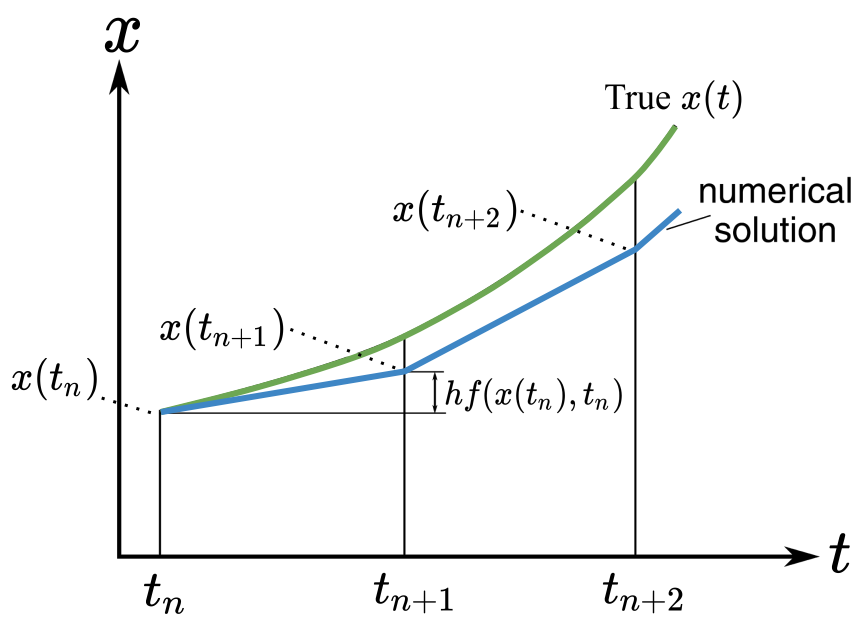
\[\frac{dx(t)}{dt} = F_{\theta}(x(t), t, \theta)\]where $x(t)$ is a feature (representation of the data) we care about (e.g., an image) and $F_{\theta}$ is a neural network with parameters $\theta$. When you are using Neural ODEs for some predictions, the ODE is solved with an ODE solver. The ODE solver solves the ODE through an iteration process. Here is the illustration of Euler’s method, a simple solver.

Another perspective to think about Neural ODEs is through looking at skip connection in Residual Networks:
\[x_{l+1} = x_{l} + s * F_{\theta}(x_l, \theta)\]where $x_l$ is the feature at layer $l$, $F_{\theta}$ is the neural network layer, $s=1$ is a variable we introduce. Under some conditions, taking $s \rightarrow 0$ would give us an ODE similar to Neural ODEs.
So Neural ODEs can be approached from two contexts: (1) parameterizing the vector field of an ODE, (2) a continous analogue of Residual Networks. Neural ODEs (and neural differential equations in general) enjoy many advantages thanks to the fresh perspective of continuous methods for machine learning. These points are elaborated in this tutorial.
Despite these new advantages, Neural ODEs can be computational expensive when the ODE solver require a large number of steps - usually referred to as the number of function evaluations (NFE) - to get good results. We are interested in reducing the NFE without sacrificing the accuracy of the model.
An optimization perspective of Neural ODEs
Gradient descent is one of the most common algorithm for optimizing some objective $F$ with respect to a variable $x$
\[\min_x F(x)\]An iteration of gradient descent is defined as follows, $x_k$ is the value of the variable $x$ at the iteration $k$
\[x_{k+1} = x_{k} - s \nabla F(x_k)\]which becomes the following ODE at the limit of $s \rightarrow 0$
\[\frac{dx}{dt} = -\nabla F(x(t))\]Comparing this with the form of Neural ODEs, we see that Neural ODEs are parameterizing the $-\nabla F(x(t))$ term with $F(x(t), t, \theta)$.
How Nesterov’s Momentum helps Neural ODEs
With this new perspective, we can use other gradient-based methods to make the ODE easier to solve, so that ODE solvers can achieve good results with a smaller number of functional evaluations. Our choice is accelerating the ODE by replacing the ODE of Neural ODEs with the Nesterov’s Accelerated Gradients ODE, which has an improved convergence rate. This Nesterov ODE is a second order ODE (which means having a second derivative instead of just the first derivative)
\[\frac{d^2x}{dt^2} + \frac{3}{t} \frac{dx}{dt} = - \nabla F(x(t))\]We modified the Nesterov ODE for better computational advantages with the following modifications:
- Converting the system to an equivalent system of first order ODEs.
- Removing the $\frac{3}{t}$ term from the differential equations through some algebraic manipulations.
The result is the following system of differential-algebraic equations (including both differential and algebraic equations), which we call Nesterov Neural ODEs (or NesterovNODEs for short).
\[\left\{ \begin{aligned} &h(t) = t^{\frac{-3}{2}}e^{\frac{t}{2}} x(t),\\ &\frac{dx(t)}{dt} = m(t),\\ &\frac{dm(t)}{dt} = -m(t) - f(h(t),t,\theta). \end{aligned} \right.\]We also create a version that is more stable for training by introducing activation functions and skip connections, called Generalized Nesterov NODEs (GNesterovNODEs). Our work also introduce differential-algebraic equations into the field of neural differential equations. This is an interesting direction because we can use algebraic equations to encode constraints into the system, which is useful for modelling physical systems that usually involve constraints such energy or momentum conservation.
Experiments
We perform extensive experiments in time series, generative modelling, and image classification to show that our model reduce the number of function evaluations without reducing accuracies.
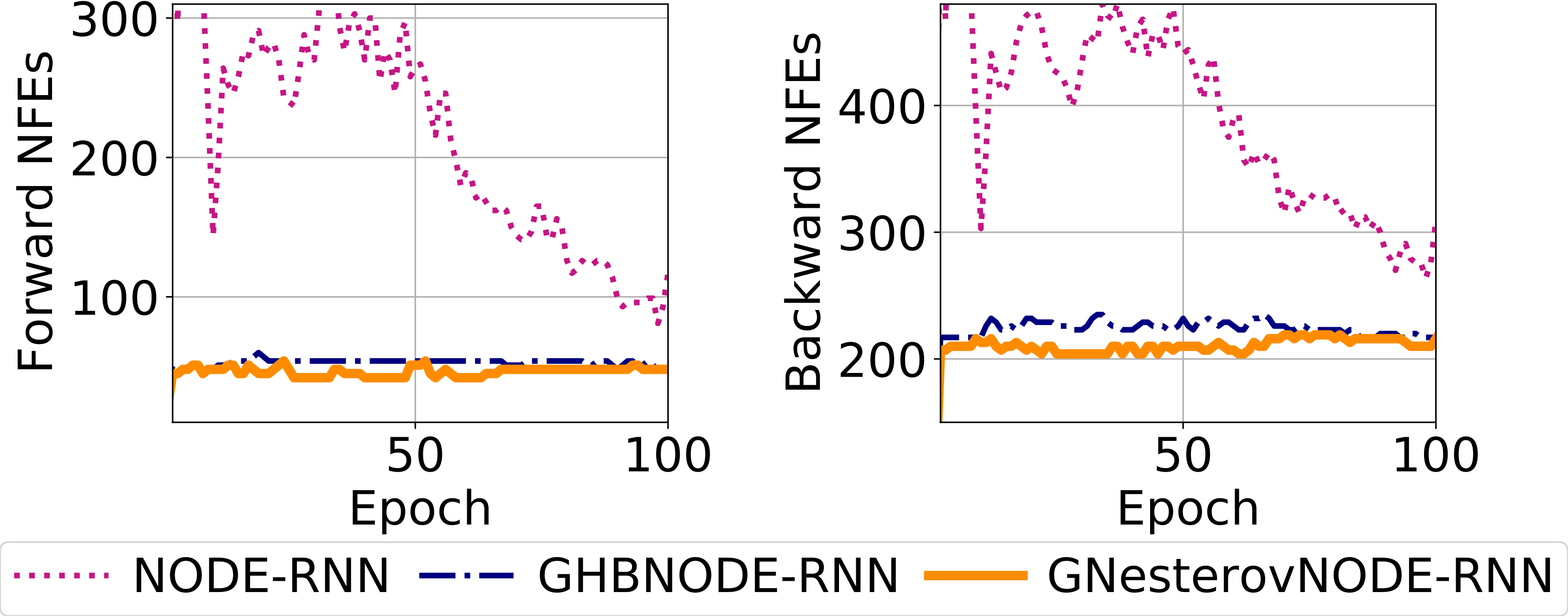
Here is the test accuracy and mean NFEs over all epochs of NODE-RNN, GHBNODE-RNN and our method GNesterovNODE-RNN on the Human Activity benchmark (Per-time-point classification).

Next, we contrast the NFEs and the validation negative ELBO of the FFJORD-NODE, the FFJORD-HBNODE, and our FFJORD-GNesterovNODE for the variational inference task with a continuous normalizing flow model, i.e. FFJORD, on the binarized MNIST dataset (generative modelling).

Next, we compare the NFEs and losses of NODE-based baselines and our methods on the Walker2D dataset (Irregular time series regresion).

Finally, we show the NFEs and accuracy of NODE-based baselines and our methods NesterovNODE/GNesterovNODE on the CIFAR10 dataset (Image classification).

Conclusion
Neural Differential Equations are a new topic in machine learning that leverage the power of differential equations for improved modeling capabilities through the power of differential equations. In our NeurIPS 2022 paper, we focus on improving the efficiency of Neural ODEs. We achieve this by introducing Nesterov’s Accelerated Gradients to Neural ODEs, which has an improved convergence rate compared to the gradient descent. We show that our model, (G)NesterovNODEs are efficient by significantly reducing the NFE without compromising the accuracy of the models compared to previous Neural ODEs based models.
